
Designing a Systolic Array Simulator: A Cycle-by-Cycle PE Model
A processing element (PE) often appears as a single multiply–accumulate symbol in a matrix multiplication diagram. Turning that symbol into a cycle-by-cycle simulator raises more specific questions. Does a neighbouring PE see the current result or the next one? How does an end-of-tile marker follow a product through a multicycle pipeline? When the dataflow changes, which values stay local and which move through the array?
This article examines a C++ PE model through its ports, state transitions, product pipeline, and dataflow support. The model separates shared timing logic from dataflow-specific computation. Following an operand from input to output makes those responsibilities easier to see.
1. The interface: three channels and a load control
The template parameters In and Acc separate operand and accumulator formats. Each data channel uses the same signal wrapper:
template<typename T>
struct Signal {
    T value{};
    bool valid = false;
    bool last = false;
};
valid indicates whether the value is meaningful. last marks the final element of the input sequence for a tile, rather than the completion of the entire matrix multiplication. It identifies the last k in output-stationary (OS) mode, the last m in weight-stationary (WS) and DIP modes, and the last n in input-stationary (IS) mode.
| Input | Type | Role in a conventional mesh |
|---|---|---|
a |
Signal<In> |
Arrives from the west and is registered before forwarding east |
b |
Signal<In> |
Arrives from the north; a streaming operand in OS, or the stationary-operand load channel in the other modes |
psum |
Signal<Acc> |
Arrives from the north and leaves south; carries partial sums or completed OS results |
load_w |
bool |
Enables loading of the stationary register |
PEOut exposes the first three channels. These directions describe a conventional two-dimensional mesh. In DIP, a enters through the top edge of the array and travels diagonally. The PE handles port values; the array determines their connections.
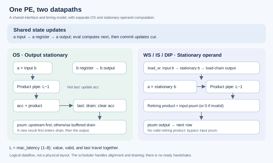
Figure 1. OS uses a local accumulator and drain buffer. WS, IS, and DIP share the stationary-operand datapath. Arrows show logical data relationships; state changes follow the eval/commit protocol.
The interface has valid signals but no ready signals. A PE cannot ask its upstream neighbour to wait through a handshake. Operand alignment, loading, and result draining are responsibilities of the scheduler.
2. Current and next state: one clock for the whole array
Updating a PE’s current state immediately while traversing an array creates a subtle problem: the PE to its right may read a value that was just computed. Data can then cross multiple PEs in one simulation step, and the result may depend on traversal order.
The model avoids this with two copies of state:
State cur_;
State next_;
| Interface | Responsibility | Externally visible state |
|---|---|---|
out() |
Returns cur_.a/b/psum |
Committed register outputs |
eval(in) |
Computes next_ from inputs and current state |
Outputs still reflect the old state |
commit() |
Assigns cur_ = next_ |
The new state becomes visible |
eval() begins with next_ = cur_, preserving fields unless the subsequent logic changes them. It then copies input a into the next state and invokes the selected dataflow logic. The copy happens regardless of valid; only valid inputs increment the corresponding register-write counter.
Each array cycle evaluates every PE before committing any of them. This mirrors synchronous hardware: combinational logic computes D, then the clock edge updates Q.
configure(mode, cfg) sets the mode and latency, then resets both state copies, statistics, and hazard counters. Reconfiguration discards in-flight products and pending results, so it must happen at a suitable computation boundary.
3. MAC latency and issue interval are different
PEConfig contains one setting:
struct PEConfig {
    int mac_latency = 1;
};
The supported range is 1–8, checked by an assertion in configure. The build configuration retains assertions in Release builds. Compiling with assertions disabled removes this check.
Product handling has two steps:
issue(x, y, last)computesmul_to<Acc>(x, y), increments the MAC counter, and creates a Product.advance(p)advances the product pipeline and returns the product reaching the accumulation stage in this cycle.
A Product carries its value, valid flag, and last flag together. The end marker therefore experiences the same delay as the arithmetic value.
The internal product pipeline has mac_latency - 1 stages. With a latency of 1, advance returns the newly issued product directly. The same eval call computes the next accumulation-related state, which becomes visible at commit. A latency of 3 adds two product-register stages ahead of that update.
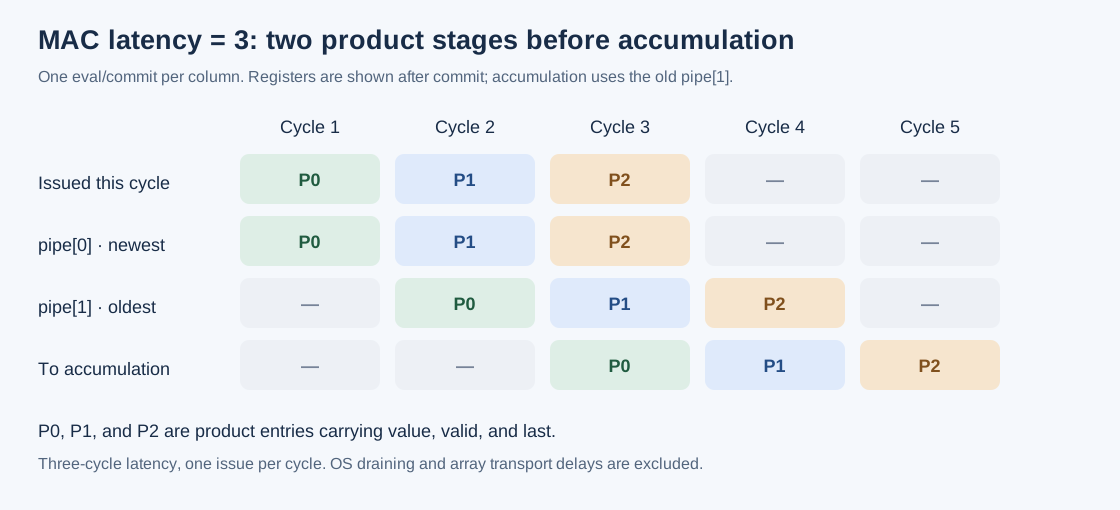
Figure 2. Each column represents one eval/commit cycle. Pipeline entries show state after commit. P0, P1, and P2 issue consecutively and reach accumulation in cycles 3, 4, and 5.
| mac_latency | Product-register stages | Accumulation state becomes visible |
|---|---|---|
| 1 | 0 | At the first commit edge after operand presentation |
| 3 | 2 | At the third commit edge |
| 8 | 7 | At the eighth commit edge |
The pipeline can accept a new product every cycle. Increasing latency does not inherently reduce the steady-state issue rate, although it increases pipeline fill and drain time.
This latency is also distinct from the array’s end-to-end latency. OS needs an additional transfer from its drain buffer to its output register, and results may still have several PE hops before leaving the array.
4. Four dataflows, two PE datapaths
The dispatch logic makes the reuse explicit:
switch (mode_) {
case Dataflow::OS:
    eval_os(in);
    break;
case Dataflow::WS:
case Dataflow::IS:
case Dataflow::DIP:
    eval_ws(in);
    break;
}
| Mode | Stationary state | Streaming operands | Main distinction |
|---|---|---|---|
| OS | Local output accumulator acc | A and B | Reduces the K dimension locally, then drains the result |
| WS | B weights in b | A | Partial sums accumulate as they travel south |
| IS | A inputs in b | B | Reuses the WS datapath with different matrix mapping |
| DIP | Permuted B weights in b | A | Reuses the WS datapath with different wiring and weight placement |
OS: accumulate locally, then join the result chain
OS issues a multiplication only when in.a.valid && in.b.valid. Both a and b are registered for forwarding.
A product reaching accumulation is added to cur_.acc. If last is false, the sum becomes the new accumulator value. If last is true, the completed sum is placed in drain and acc is cleared for the next tile.
The psum output follows this priority:
- Forward a valid incoming psum from the PE above.
- Otherwise, send a valid result already held in cur_.drain and clear that buffer.
- If neither source is valid, produce an invalid output.
A result completed in the current cycle therefore does not immediately appear on out().psum. It enters drain at commit and can reach the output register in the following cycle at the earliest.
If a new result completes before the old drain entry has been released, the model increments drain_overflow and overwrites the buffer. This counter reports a scheduling conflict; it does not provide backpressure or extra queue capacity.
WS: keep one operand local and move the partial sum
When load_w is asserted, the PE assigns next_.b = in.b. Otherwise, b holds its value. The stationary register is also the load-chain register; there is no shadow copy for the next set of weights.
Whenever in.a.valid is true, the multiplication uses the streaming operand and cur_.b.value. If a load happens in the same cycle, multiplication still uses the old stationary value. The model increments load_hazard when loading coincides with a valid a input, but computation continues.
Issue also does not check cur_.b.valid. The scheduler must ensure that the correct stationary value has been loaded before sending an activation.
When a product reaches accumulation, it is added to the incoming partial sum:
Acc base = in.psum.valid ? in.psum.value : Acc{};
next_.psum = {base + r.value, true, r.last};
If no valid product retires, the PE forwards in.psum directly. This decision depends on r.valid at the pipeline exit: a bubble at the current input does not imply that the pipeline has no product to accumulate.
IS and DIP: change mapping and wiring
IS loads A into the stationary registers and streams B through the array. Despite its name, load_w therefore controls input loading in this mode.
DIP changes the array topology and schedule. A enters the top edge without skew, then moves down one row and left one column per cycle, wrapping at the boundary. Weights are permuted to match the resulting k order. This implementation requires a square array, while each PE still executes eval_ws.
All three stationary-operand modes must avoid reloading too early. The scheduler inserts barriers between tiles and waits for the preceding tile’s results to drain before starting the next load.
5. Numeric precision is part of the behaviour
Separating In from Acc allows operand format and accumulator width to vary independently. The model supports seven explicitly instantiated combinations:
| Input | Accumulator | Arithmetic behaviour |
|---|---|---|
| int8_t | 16-bit or 32-bit SInt | Wrap or saturate at either width |
| int16_t | 48-bit SInt | Wrap or saturate |
| BF16 | float | BF16 storage with FP32 products and accumulation |
The mul_to function converts the product to Acc at issue time. Subsequent additions follow that type’s arithmetic rules. Narrow product conversion, intermediate saturation, and wraparound can all affect the result; a single conversion at the final output cannot generally reproduce them.
FP32-to-BF16 conversion uses round-to-nearest-even. The PE source computes a product and then adds it, without explicitly calling std::fma. Matching a particular hardware floating-point implementation also requires checking compiler options and the target arithmetic rules.
Explicit template instantiation generates these supported implementations. Adding a precision requires updating the type-combination list and, if runtime selection is needed, the precision registry.
6. Counters measure events, not just busy cycles
PEStats records more than multiplication counts:
| Counter | Meaning |
|---|---|
| mac | Calls to issue: the number of multiplications issued |
| idle | Cycles with no new operand pair issued |
| reg_a_wr | Register writes for valid a inputs |
| reg_b_wr | Register writes for valid b inputs in OS |
| w_load | Valid stationary-value writes during loading |
| psum_wr | Acc-width write events for accumulation-related state, completed-result buffering, and psum output |
| pipe_wr | Valid-entry writes across the product pipeline stages |
With one eval/commit per cycle, each PE satisfies $\mathrm{mac} + \mathrm{idle} = \mathrm{cycles}$. However, an idle cycle can still advance an older product, update an accumulated sum, or forward a result.
psum_wr may increase more than once in a cycle. So may pipe_wr when several stages contain valid products. Invalid inputs still update validity state, but the counters do not attempt to capture every physical bit transition. They represent the event costs defined by the model.
The energy_pj function applies a linear estimate:
\[\begin{aligned} \mathrm{register\_bits} &= (\mathrm{reg\_a\_wr} + \mathrm{reg\_b\_wr} + \mathrm{w\_load}) \\ &\quad \times \mathrm{input\_bits} \\ &\quad + (\mathrm{psum\_wr} + \mathrm{pipe\_wr}) \\ &\quad \times \mathrm{accumulator\_bits} \end{aligned}\] \[\begin{aligned} \mathrm{energy\_pJ} &= \mathrm{mac} \times E_{\mathrm{mac}} \\ &\quad + \mathrm{register\_bits} \times E_{\mathrm{reg\_bit}} \\ &\quad + \mathrm{idle} \times E_{\mathrm{idle}} \end{aligned}\]BitWidth
This estimate is useful for comparing PE event costs under consistent coefficients. It does not separately account for valid/last metadata, interconnect, SRAM, or the full clock tree. EnergyModel defaults to zero coefficients, and some simulator parameters are placeholders. Credible absolute energy estimates require calibration against the target process or synthesis results.
7. A three-cycle example
Consider an OS PE computing $2\times 3 + 4\times 5 = 26$, with a MAC latency of 1 and no incoming result occupying its output chain:
| Cycle | Input | acc after commit | drain after commit | psum after commit |
|---|---|---|---|---|
| 1 | a=2, b=3, last=false | 6 | Invalid | Invalid |
| 2 | a=4, b=5, a.last=true | 0 | 26, valid | Invalid |
| 3 | No valid operands | 0 | Invalid | 26, valid |
Arithmetic completes in cycle 2, but the output becomes visible in cycle 3. Cycle 3 increments idle while still performing a useful transfer. OS takes the end marker from in.a.last without checking that a.last and b.last agree, so the scheduler must enforce that protocol.
The following fragment illustrates the calling sequence. AccI32W denotes a signed 32-bit wrapping accumulator; the example depends on the model’s type definitions and implementation.
// Configure, evaluate the next state, then commit.
PE<int8_t, AccI32W> pe;
pe.configure(Dataflow::OS, PEConfig{1});

PEIn<int8_t, AccI32W> in;
in.a = {int8_t{2}, true, false};
in.b = {int8_t{3}, true, false};
pe.eval(in);          // out() still returns the old register state.
pe.commit();         // acc() is now 6.
The design assigns local arithmetic and state to the PE, connections to the array, and operand timing and draining to the scheduler. To interpret cycle counts and utilisation, check that all PEs evaluate before any commit, verify loading and last-marker alignment, and distinguish arithmetic completion from the moment a result leaves the array.
The diagrams and examples follow the model’s state-transition rules; they are not measured hardware performance results. A reference calculation using the same numeric rules and reduction order can check arithmetic, while hazard counters and cycle traces help locate timing errors.